Bayesian Regression
import numpy as np
import matplotlib.pyplot as plt
import seaborn as sns
from sklearn import datasets
boston = datasets.load_boston()
X = boston['data']
y = boston['target']
The BayesianRegression class estimates the regression coefficients using
Note that this assumes \(\sigma^2\) and \(\tau\) are known. We can determine the influence of the prior distribution by manipulationg \(\tau\), though there are principled ways to choose \(\tau\). There are also principled Bayesian methods to model \(\sigma^2\) (see here), though for simplicity we will estimate it with the typical OLS estimate:
where \(SSE\) is the sum of squared errors from an ordinary linear regression, \(N\) is the number of observations, and \(D\) is the number of predictors. Using the linear regression model from chapter 1, this comes out to about 11.8.
class BayesianRegression:

    def fit(self, X, y, sigma_squared, tau, add_intercept = True):

        # record info
        if add_intercept:
            ones = np.ones(len(X)).reshape((len(X),1))
            X = np.append(ones, np.array(X), axis = 1)
        self.X = X
        self.y = y

        # fit
        XtX = np.dot(X.T, X)/sigma_squared
        I = np.eye(X.shape[1])/tau
        inverse = np.linalg.inv(XtX + I)
        Xty = np.dot(X.T, y)/sigma_squared
        self.beta_hats = np.dot(inverse , Xty)

        # fitted values
        self.y_hat = np.dot(X, self.beta_hats)
Let’s fit a Bayesian regression model on the Boston housing dataset. We’ll use \(\sigma^2 = 11.8\) and \(\tau = 10\).
sigma_squared = 11.8
tau = 10
model = BayesianRegression()
model.fit(X, y, sigma_squared, tau)
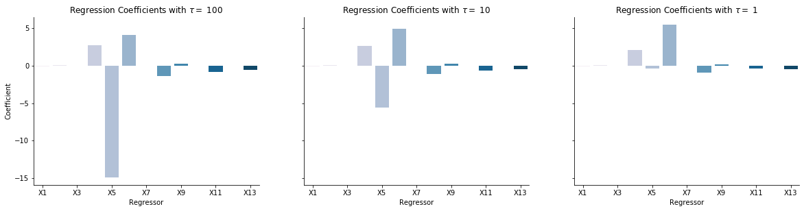
The below plot shows the estimated coefficients for varying levels of \(\tau\). A lower value of \(\tau\) indicates a stronger prior, and therefore a greater pull of the coefficients towards their expected value (in this case, 0). As expected, the estimates approach 0 as \(\tau\) decreases.
Xs = ['X'+str(i + 1) for i in range(X.shape[1])]
taus = [100, 10, 1]

fig, ax = plt.subplots(ncols = len(taus), figsize = (20, 4.5), sharey = True)
for i, tau in enumerate(taus):
    model = BayesianRegression()
    model.fit(X, y, sigma_squared, tau)
    betas = model.beta_hats[1:]
    sns.barplot(Xs, betas, ax = ax[i], palette = 'PuBu')
    ax[i].set(xlabel = 'Regressor', title = fr'Regression Coefficients with $\tau = $ {tau}')
    ax[i].set(xticks = np.arange(0, len(Xs), 2), xticklabels = Xs[::2])

ax[0].set(ylabel = 'Coefficient')
sns.set_context("talk")
sns.despine();