Common Methods
This section will review two methods that are used to fit a variety of machine learning models: gradient descent and cross validation. These methods will be used repeatedly throughout this book.
1. Gradient Descent
Almost all the models discussed in this book aim to find a set of parameters that minimize a chosen loss function. Sometimes we can find the optimal parameters by taking the derivative of the loss function, setting it equal to 0, and solving. In situations for which no closed-form solution is available, however, we might turn to gradient descent. Gradient descent is an iterative approach to approximating the parameters that minimize a differentiable loss function.
The Set-Up
Let’s first introduce a typical set-up for gradient descent. Suppose we have \(N\) observations where each observation has predictors \(\bx_n\) and target variable \(y_n\). We decide to approximate \(y_n\) with \(\hat{y}_n = f(\bx_n, \bbetahat)\), where \(f()\) is some differentiable function and \(\bbetahat\) is a set of parameter estimates. Next, we introduce a differentiable loss function \(\mathcal{L}\). For simplicity, let’s assume we can write the model’s entire loss as the sum of the individual losses across observations. That is,
where \(g()\) is some differentiable function representing an observation’s individual loss.
To fit this generic model, we want to find the values of \(\bbetahat\) that minimize \(\mathcal{L}\). We will likely start with the following derivative:
Ideally, we can set the above derivative equal to 0 and solve for \(\bbetahat\), giving our optimal solution. If this isn’t possible, we can iteratively search for the values of \(\bbetahat\) that minimize \(\mathcal{L}\). This is the process of gradient descent.
An Intuitive Introduction
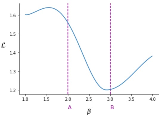
To understand this process intuitively, consider the image above showing a model’s loss as a function of one parameter, \(\beta\). We start our search for the optimal \(\beta\) by randomly picking a value. Suppose we start with \(\beta\) at point \(A\). From point \(A\) we ask “would the loss function decrease if I increased or decreased \(\beta\)”. To answer this question, we calculate the derivative of \(\mathcal{L}\) with respect to \(\beta\) evaluated at \(\beta = A\). Since this derivative is negative, we know that increasing \(\beta\) some small amount will decrease the loss.
Now we know we want to increase \(\beta\), but how much? Intuitively, the more negative the derivative, the more the loss will decrease with an increase in \(\beta\). So, let’s increase \(\beta\) by an amount proportional to the negative of the derivative. Letting \(\delta\) be the derivative and \(\eta\) be a small constant learning rate, we might increase \(\beta\) with
The more negative \(\delta\) is, the more we increase \(\beta\).
Now suppose we make the increase and wind up with \(\beta = B\). Calculating the derivative again, we get a slightly positive number. This tells us that we went too far: increasing \(\beta\) will increase \(\mathcal{L}\). However, since the derivative is only slightly positive, we want to only make a slight correction. Let’s again use the same adjustment, \(\beta \gets \beta - \eta\delta\). Since \(\delta\) is now slightly positive, \(\beta\) will now decrease slightly. We will repeat this same process a fixed number of times or until \(\beta\) barely changes. And that is gradient descent!
The Steps
We can describe gradient descent more concretely with the following steps. Note here that \(\bbetahat\) can be a vector, rather than just a single parameter.
Choose a small learning rate \(\eta\)
Randomly instantiate \(\bbetahat\)
For a fixed number of iterations or until some stopping rule is reached:
Calculate \(\boldsymbol{\delta} = \partial \mathcal{L}/\partial \bbetahat\)
Adjust \(\bbetahat\) with
\[ \bbetahat \gets \bbetahat - \eta \boldsymbol{\delta}. \]
A potential stopping rule might be a minimum change in the magnitude of \(\bbetahat\) or a minimum decrease in the loss function \(\mathcal{L}\).
An Example
As a simple example of gradient descent in action, let’s derive the ordinary least squares (OLS) regression estimates. (This problem does have a closed-form solution, but we’ll use gradient descent to demonstrate the approach). As discussed in Chapter 1, linear regression models \(\hat{y}_n\) with
where \(\bx_n\) is a vector of predictors appended with a leading 1 and \(\bbetahat\) is a vector of coefficients. The OLS loss function is defined with
After choosing \(\eta\) and randomly instantiating \(\bbetahat\), we iteratively calculate the loss function’s gradient:
and adjust with
This is accomplished with the following code. Note that we can also calculate \(\boldsymbol{\delta} = -\bX^\top(\by - \hat{\by})\), where \(\bX\) is the feature matrix, \(\by\) is the vector of targets, and \(\hat{\by}\) is the vector of fitted values.
import numpy as np

def OLS_GD(X, y, eta = 1e-3, n_iter = 1e4, add_intercept = True):

  ## Add Intercept
  if add_intercept:
    ones = np.ones(X.shape[0]).reshape(-1, 1)
    X = np.concatenate((ones, X), 1)

  ## Instantiate
  beta_hat = np.random.randn(X.shape[1])

  ## Iterate
  for i in range(int(n_iter)):

    ## Calculate Derivative
    yhat = X @ beta_hat
    delta = -X.T @ (y - yhat)
    beta_hat -= delta*eta
2. Cross Validation
Several of the models covered in this book require hyperparameters to be chosen exogenously (i.e. before the model is fit). The value of these hyperparameters affects the quality of the model’s fit. So how can we choose these values without fitting a model? The most common answer is cross validation.
Suppose we are deciding between several values of a hyperparameter, resulting in multiple competing models. One way to choose our model would be to split our data into a training set and a validation set, build each model on the training set, and see which performs better on the validation set. By splitting the data into training and validation, we avoid evaluating a model based on its in-sample performance.
The obvious problem with this set-up is that we are comparing the performance of models on just one dataset. Instead, we might choose between competing models with K-fold cross validation, outlined below.
Split the original dataset into \(K\) folds or subsets.
For \(k = 1, \dots, K\), treat fold \(k\) as the validation set. Train each competing model on the data from the other \(K-1\) folds and evaluate it on the data from the \(k^\text{th}\).
Select the model with the best average validation performance.
As an example, let’s use cross validation to choose a penalty value for a Ridge regression model, discussed in chapter 2. This model constrains the magnitude of the regression coefficients; the higher the penalty term, the more the coefficients are constrained.
The example below uses the Ridge class from scikit-learn, which defines the penalty term with the alpha argument. We will use the Boston housing dataset.
## Import packages
import numpy as np
from sklearn.linear_model import Ridge
from sklearn.datasets import load_boston

## Import data
boston = load_boston()
X = boston['data']
y = boston['target']
N = X.shape[0]

## Choose alphas to consider
potential_alphas = [0, 1, 10]
error_by_alpha = np.zeros(len(potential_alphas))

## Choose the folds
K = 5
indices = np.arange(N)
np.random.shuffle(indices)
folds = np.array_split(indices, K)

## Iterate through folds
for k in range(K):

  ## Split Train and Validation
    X_train = np.delete(X, folds[k], 0)
    y_train = np.delete(y, folds[k], 0)
    X_val = X[folds[k]]
    y_val = y[folds[k]]

  ## Iterate through Alphas
    for i in range(len(potential_alphas)):

        ## Train on Training Set
        model = Ridge(alpha = potential_alphas[i])
        model.fit(X_train, y_train)

        ## Calculate and Append Error
        error = np.sum( (y_val - model.predict(X_val))**2 )
        error_by_alpha[i] += error

error_by_alpha /= N
We can then check error_by_alpha and choose the alpha corresponding to the lowest average error!