Concept
Model Structure
Linear regression is a relatively simple method that is extremely widely-used. It is also a great stepping stone for more sophisticated methods, making it a natural algorithm to study first.
In linear regression, the target variable \(y\) is assumed to follow a linear function of one or more predictor variables, \(x_1, \dots, x_D\), plus some random error. Specifically, we assume the model for the \(n^\text{th}\) observation in our sample is of the form
Here \(\beta_0\) is the intercept term, \(\beta_1\) through \(\beta_D\) are the coefficients on our feature variables, and \(\epsilon\) is an error term that represents the difference between the true \(y\) value and the linear function of the predictors. Note that the terms with an \(n\) in the subscript differ between observations while the terms without (namely the \(\beta\text{s}\)) do not.
The math behind linear regression often becomes easier when we use vectors to represent our predictors and coefficients. Let’s define \(\bx_n\) and \(\bbeta\) as follows:
Note that \(\bx_n\) includes a leading 1, corresponding to the intercept term \(\beta_0\). Using these definitions, we can equivalently express \(y_n\) as
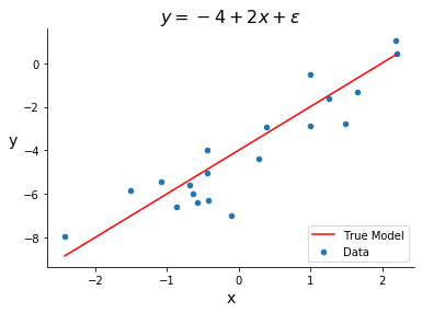
Below is an example of a dataset designed for linear regression. The input variable is generated randomly and the target variable is generated as a linear combination of that input variable plus an error term.
import numpy as np
import matplotlib.pyplot as plt
import seaborn as sns

# generate data
np.random.seed(123)
N = 20
beta0 = -4
beta1 = 2
x = np.random.randn(N)
e = np.random.randn(N)
y = beta0 + beta1*x + e
true_x = np.linspace(min(x), max(x), 100)
true_y = beta0 + beta1*true_x

# plot
fig, ax = plt.subplots()
sns.scatterplot(x, y, s = 40, label = 'Data')
sns.lineplot(true_x, true_y, color = 'red', label = 'True Model')
ax.set_xlabel('x', fontsize = 14)
ax.set_title(fr"$y = {beta0} + ${beta1}$x + \epsilon$", fontsize = 16)
ax.set_ylabel('y', fontsize=14, rotation=0, labelpad=10)
ax.legend(loc = 4)
sns.despine()
Parameter Estimation
The previous section covers the entire structure we assume our data follows in linear regression. The machine learning task is then to estimate the parameters in \(\bbeta\). These estimates are represented by \(\hat{\beta}_0, \dots, \hat{\beta}_D\) or \(\bbetahat\). The estimates give us fitted values for our target variable, represented by \(\hat{y}_n\).
This task can be accomplished in two ways which, though slightly different conceptually, are identical mathematically. The first approach is through the lens of minimizing loss. A common practice in machine learning is to choose a loss function that defines how well a model with a given set of parameter estimates the observed data. The most common loss function for linear regression is squared error loss. This says the loss of our model is proportional to the sum of squared differences between the true \(y_n\) values and the fitted values, \(\hat{y}_n\). We then fit the model by finding the estimates \(\bbetahat\) that minimize this loss function. This approach is covered in the subsection Approach 1: Minimizing Loss.
The second approach is through the lens of maximizing likelihood. Another common practice in machine learning is to model the target as a random variable whose distribution depends on one or more parameters, and then find the parameters that maximize its likelihood. Under this approach, we will represent the target with \(Y_n\) since we are treating it as a random variable. The most common model for \(Y_n\) in linear regression is a Normal random variable with mean \(E(Y_n) = \bbeta^\top \bx_n\). That is, we assume
and we find the values of \(\bbetahat\) to maximize the likelihood. This approach is covered in subsection Approach 2: Maximizing Likelihood.
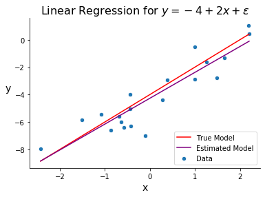
Once we’ve estimated \(\bbeta\), our model is fit and we can make predictions. The below graph is the same as the one above but includes our estimated line-of-best-fit, obtained by calculating \(\hat{\beta}_0\) and \(\hat{\beta}_1\).
# generate data
np.random.seed(123)
N = 20
beta0 = -4
beta1 = 2
x = np.random.randn(N)
e = np.random.randn(N)
y = beta0 + beta1*x + e
true_x = np.linspace(min(x), max(x), 100)
true_y = beta0 + beta1*true_x

# estimate model
beta1_hat = sum((x - np.mean(x))*(y - np.mean(y)))/sum((x - np.mean(x))**2)
beta0_hat = np.mean(y) - beta1_hat*np.mean(x)
fit_y = beta0_hat + beta1_hat*true_x

# plot
fig, ax = plt.subplots()
sns.scatterplot(x, y, s = 40, label = 'Data')
sns.lineplot(true_x, true_y, color = 'red', label = 'True Model')
sns.lineplot(true_x, fit_y, color = 'purple', label = 'Estimated Model')
ax.set_xlabel('x', fontsize = 14)
ax.set_title(fr"Linear Regression for $y = {beta0} + ${beta1}$x + \epsilon$", fontsize = 16)
ax.set_ylabel('y', fontsize=14, rotation=0, labelpad=10)
ax.legend(loc = 4)
sns.despine()
Extensions of Ordinary Linear Regression
There are many important extensions to linear regression which make the model more flexible. Those include Regularized Regression—which balances the bias-variance tradeoff for high-dimensional regression models—Bayesian Regression—which allows for prior distributions on the coefficients—and GLMs—which introduce non-linearity to regression models. These extensions are discussed in the next chapter.