Probability¶

Many machine learning methods are rooted in probability theory. Probabilistic methods in this book include linear regression, Bayesian regression, and generative classifiers. This section covers the probability theory needed to understand those methods.

1. Random Variables and Distributions¶

Random Variables¶

A random variable is a variable whose value is randomly determined. The set of possible values a random variable can take on is called the variable’s support. An example of a random variable is the value on a die roll. This variable’s support is \(\{1, 2, 3, 4, 5, 6\}\). Random variables will be represented with uppercase letters and values in their support with lowercase letters. For instance \(X = x\) implies that a random variable \(X\) happened to take on value \(x\). Letting \(X\) be the value of a die roll, \(X = 4\) indicates that the die landed on 4.

Density Functions¶

The likelihood that a random variable takes on a given value is determined through its density function. For a discrete random variable (one that can take on a finite set of values), this density function is called the probability mass function (PMF). The PMF of a random variable \(X\) gives the probability that \(X\) will equal some value \(x\). We write it as \(f_X(x)\) or just \(f(x)\), and it is defined as

\[ f(x) = P(X = x). \]

For a continuous random variable (one that can take on infinitely many values), the density function is called the probability density function (PDF). The PDF \(f_X(x)\) of a continuous random variable \(X\) does not give \(P(X = x)\) but it does determine the probability that \(X\) lands in a certain range. Specifically,

\[ P(a \leq X \leq b) = \int_{x = a}^b f(x) dx. \]

That is, integrating \(f(x)\) over a certain range gives the probability of \(X\) being in that range. While \(f(x)\) does not give the probability that \(X\) will equal a certain value, it does indicate the relative likelihood that it will be around that value. E.g. if \(f(a) > f(b)\), we can say \(X\) is more likely to be in an arbitrarily small area around the value \(a\) than around the value \(b\).

Distributions¶

A random variable’s distribution is determined by its density function. Variables with the same density function are said to follow the same distributions. Certain families of distributions are very common in probability and machine learning. Two examples are given below.

The Bernoulli distribution is the most simple probability distribution and it describes the likelihood of the outcomes of a binary event. Let \(X\) be a random variable that equals 1 (representing “success”) with probability \(p\) and 0 (representing “failure”) with probability \(1-p\). Then, \(X\) is said to follow the Bernoulli distribution with probability parameter \(p\), written \(X \sim \text{Bern}(p)\), and its PMF is given by

\[ f_X(x) = p^x(1-p)^{(1-x)}. \]

We can check to see that for any valid value \(x\) in the support of \(X\)—i.e., 1 or 0—, \(f(x)\) gives \(P(X = x)\).

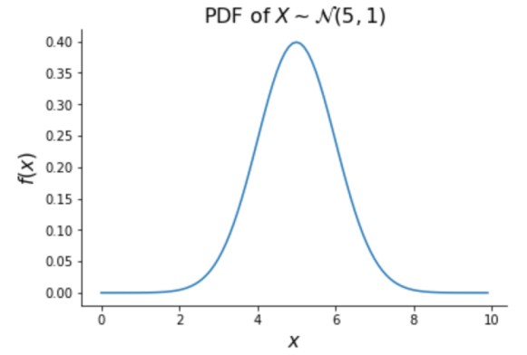
The Normal distribution is extremely common and will be used throughout this book. A random variable \(X\) follows the Normal distribution with mean parameter \(\mu \in \R\) and variance parameter \(\sigma^2 > 0\), written \(X \sim \mathcal{N}(\mu, \sigma^2)\), if its PDF is defined as

\[ f(x) = \frac{1}{\sqrt{2\pi\sigma^2}}e^{-\frac{(x-\mu)^2}{2\sigma^2}}. \]

The shape of the Normal random variable’s density function gives this distribution the name “the bell curve”, as shown below. Values closest to \(\mu\) are most likely and the density is symmetric around \(\mu\).

normal

Independence¶

So far we’ve discussed the density of individual random variables. The picture can get much more complicated when we want to study the behavior of multiple random variables simultaneously. The assumption of independence simplifies things greatly. Let’s start by defining independence in the discrete case.

Two discrete random variables \(X\) and \(Y\) are independent if and only if

\[ P(X = x, Y =y) = P(X = x)P(Y = y), \]

for all \(x\) and \(y\). This says that if \(X\) and \(Y\) are independent, the probability that \(X = x\) and \(Y = y\) simultaneously is just the product of the probabilities that \(X = x\) and \(Y = y\) individually.

To generalize this definition to continuous random variables, let’s first introduce joint density function. Quite simply, the joint density of two random variables \(X\) and \(Y\), written \(f_{X, Y}(x, y)\) gives the probability density of \(X\) and \(Y\) evaluated simultaneously at \(x\) and \(y\), respectively. We can then say that \(X\) and \(Y\) are independent if and only if

\[ f_{X, Y}(x, y) = f_X(x) f_Y(y), \]

for all \(x\) and \(y\).

2. Maximum Likelihood Estimation¶

Maximum likelihood estimation is used to understand the parameters of a distribution that gave rise to observed data. In order to model a data generating process, we often assume it comes from some family of distributions, such as the Bernoulli or Normal distributions. These distributions are indexed by certain parameters (\(p\) for the Bernoulli and \(\mu\) and \(\sigma^2\) for the Normal)—maximum likelihood estimation evaluates which parameters would be most consistent with the data we observed.

Specifically, maximum likelihood estimation finds the values of unknown parameters that maximize the probability of observing the data we did. Basic maximum likelihood estimation can be broken into three steps:

Find the joint density of the observed data, also called the likelihood
Take the log of the likelihood, giving the log-likelihood.
Find the value of the parameter that maximizes the log-likelihood (and therefore the likelihood as well) by setting its derivative equal to 0.

Finding the value of the parameter to maximize the log-likelihood rather than the likelihood makes the math easier and gives us the same solution.

Let’s go through an example. Suppose we are interested in calculating the average weight of a Chihuahua. We assume the weight of any given Chihuahua is independently distributed Normally with \(\sigma^2 = 1\) but an unknown mean \(\mu\). So, we gather 10 Chihuahuas and weigh them. Denote the \(j^\text{th}\) Chihuahua weight with \(W_j \sim \mathcal{N}(\mu, 1)\). For step 1, let’s calculate the probability density of our data (i.e., the 10 Chihuahua weights). Since the weights are assumed to be independent, the densities multiply. Letting \(L(\mu)\) be the likelihood of \(\mu\), we have

\[\begin{split} \begin{align} L(\mu) &= f_{W_1, \dots, W_{10}}(w_1, \dots, w_{10}) \\ &= f_{W_1}(w_1)\cdot...\cdot f_{W_{10}}(w_{10}) \\ &= \prod_{j = 1}^{10} \frac{1}{\sqrt{2\pi\cdot 1}}\exp\left(-\frac{(w_j - \mu)^2}{2} \right) \\ &\propto \exp\left(-\sum_{j = 1}^{10}\frac{(w_j - \mu)^2}{2} \right). \\ \end{align} \end{split}\]

Note that we can work up to a constant of proportionality since the value of \(\mu\) that maximizes \(L(\mu)\) will also maximize anything proportional to \(L(\mu)\). For step 2, take the log:

\[ \log L(\mu) = -\sum_{j = 1}^{10}\frac{(w_j - \mu)^2}{2} + c, \]

where \(c\) is some constant. For step 3, take the derivative:

\[ \begin{align} \frac{\partial}{\partial \mu}\log L(\mu) = -\sum_{j = 1}^{10}(w_j - \mu). \end{align} \]

Setting this equal to 0, we find that the (log) likelihood is maximized with

\[ \hat{\mu} = \frac{1}{10}\sum_{j = 1}^{10} w_j = \bar{w}. \]

We put a hat over \(\mu\) to indicate that it is our estimate of the true \(\mu\). Note the sensible result—we estimate the true mean of the Chihuahua weight distribution to be the sample mean of our observed data.

3. Conditional Probability¶

Probabilistic machine learning methods typically consider the distribution of a target variable conditional on the value of one or more predictor variables. To understand these methods, let’s introduce some of the basic principles of conditional probability.

Consider two events, \(A\) and \(B\). The conditional probability of \(A\) given \(B\) is the probability that \(A\) occurs given \(B\) occurs, written \(P(A|B)\). Closely related is the joint probability of \(A\) and \(B\), or the probability that both \(A\) and \(B\) occur, written \(P(A, B)\). We navigate between the conditional and joint probability with the following

\[ P(A, B) = P(A|B)P(B). \]

The above equation leads to an extremely important principle in conditional probability: Bayes’ rule. Bayes’ rule states that

\[ P(A|B) = \frac{P(B|A)P(A)}{P(B)}. \]

Both of the above expressions work for random variables as well as events. For any two discrete random variables, \(X\) and \(Y\)

\[\begin{split} \begin{align} P(X = x, Y = y) &= P(X = x|Y = y)P(Y = y) \\ P(X = x|Y = y) &= \frac{P(Y = y|X = x)P(X = x)}{P(Y = y)}. \end{align} \end{split}\]

The same is true for continuous random variables, replacing the PMFs with PDFs.

Machine Learning from Scratch