Implementation
This section demonstrates how to fit a regression model in Python in practice. The two most common packages for fitting regression models in Python are scikit-learn and statsmodels. Both methods are shown before.
First, let’s import the data and necessary packages. We’ll again be using the Boston housing dataset from sklearn.datasets.
import matplotlib.pyplot as plt
import seaborn as sns
from sklearn import datasets
boston = datasets.load_boston()
X_train = boston['data']
y_train = boston['target']
Scikit-Learn
Fitting the model in scikit-learn is very similar to how we fit our model from scratch in the previous section. The model is fit in two steps: first instantiate the model and second use the fit() method to train it.
from sklearn.linear_model import LinearRegression
sklearn_model = LinearRegression()
sklearn_model.fit(X_train, y_train);
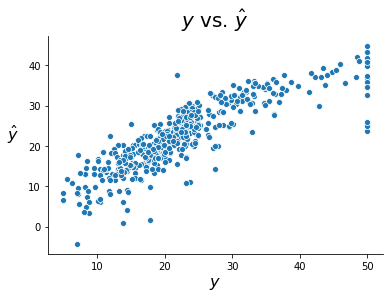
As before, we can plot our fitted values against the true values. To form predictions with the scikit-learn model, we can use the predict method. Reassuringly, we get the same plot as before.
sklearn_predictions = sklearn_model.predict(X_train)
fig, ax = plt.subplots()
sns.scatterplot(y_train, sklearn_predictions)
ax.set_xlabel(r'$y$', size = 16)
ax.set_ylabel(r'$\hat{y}$', rotation = 0, size = 16, labelpad = 15)
ax.set_title(r'$y$ vs. $\hat{y}$', size = 20, pad = 10)
sns.despine()
We can also check the estimated parameters using the coef_ attribute as follows (note that only the first few are printed).
predictors = boston.feature_names
beta_hats = sklearn_model.coef_
print('\n'.join([f'{predictors[i]}: {round(beta_hats[i], 3)}' for i in range(3)]))
CRIM: -0.108
ZN: 0.046
INDUS: 0.021
Statsmodels
statsmodels is another package frequently used for running linear regression in Python. There are two ways to run regression in statsmodels. The first uses numpy arrays like we did in the previous section. An example is given below.
Note
Note two subtle differences between this model and the models we’ve previously built. First, we have to manually add a constant to the predictor dataframe in order to give our model an intercept term. Second, we supply the training data when instantiating the model, rather than when fitting it.
import statsmodels.api as sm

X_train_with_constant = sm.add_constant(X_train)
sm_model1 = sm.OLS(y_train, X_train_with_constant)
sm_fit1 = sm_model1.fit()
sm_predictions1 = sm_fit1.predict(X_train_with_constant)
The second way to run regression in statsmodels is with R-style formulas and pandas dataframes. This allows us to identify predictors and target variables by name. An example is given below.
import pandas as pd
df = pd.DataFrame(X_train, columns = boston['feature_names'])
df['target'] = y_train
display(df.head())

formula = 'target ~ ' + ' + '.join(boston['feature_names'])
print('formula:', formula)
| CRIM | ZN | INDUS | CHAS | NOX | RM | AGE | DIS | RAD | TAX | PTRATIO | B | LSTAT | target | |
|---|---|---|---|---|---|---|---|---|---|---|---|---|---|---|
| 0 | 0.00632 | 18.0 | 2.31 | 0.0 | 0.538 | 6.575 | 65.2 | 4.0900 | 1.0 | 296.0 | 15.3 | 396.90 | 4.98 | 24.0 |
| 1 | 0.02731 | 0.0 | 7.07 | 0.0 | 0.469 | 6.421 | 78.9 | 4.9671 | 2.0 | 242.0 | 17.8 | 396.90 | 9.14 | 21.6 |
| 2 | 0.02729 | 0.0 | 7.07 | 0.0 | 0.469 | 7.185 | 61.1 | 4.9671 | 2.0 | 242.0 | 17.8 | 392.83 | 4.03 | 34.7 |
| 3 | 0.03237 | 0.0 | 2.18 | 0.0 | 0.458 | 6.998 | 45.8 | 6.0622 | 3.0 | 222.0 | 18.7 | 394.63 | 2.94 | 33.4 |
| 4 | 0.06905 | 0.0 | 2.18 | 0.0 | 0.458 | 7.147 | 54.2 | 6.0622 | 3.0 | 222.0 | 18.7 | 396.90 | 5.33 | 36.2 |
formula: target ~ CRIM + ZN + INDUS + CHAS + NOX + RM + AGE + DIS + RAD + TAX + PTRATIO + B + LSTAT
import statsmodels.formula.api as smf

sm_model2 = smf.ols(formula, data = df)
sm_fit2 = sm_model2.fit()
sm_predictions2 = sm_fit2.predict(df)