Logistic Regression
import numpy as np
np.set_printoptions(suppress=True)
import matplotlib.pyplot as plt
import seaborn as sns
from sklearn import datasets
In this section we will construct binary and multiclass logistic regression models. We will try our binary model on the breast cancer dataset and the multiclass model on the wine dataset.
Binary Logistic Regression
# import data
cancer = datasets.load_breast_cancer()
X = cancer['data']
y = cancer['target']
Let’s first define some helper functions: the logistic function and a standardization function, equivalent to scikit-learn’s StandardScaler
def logistic(z):
    return (1 + np.exp(-z))**(-1)

def standard_scaler(X):
    mean = X.mean(0)
    sd = X.std(0)
    return (X - mean)/sd
The binary logistic regression class is defined below. First, it (optionally) standardizes and adds an intercept term. Then it estimates \(\boldsymbol{\beta}\) with gradient descent, using the gradient of the negative log-likelihood derived in the concept section,
class BinaryLogisticRegression:

    def fit(self, X, y, n_iter, lr, standardize = True, has_intercept = False):

        ### Record Info ###
        if standardize:
            X = standard_scaler(X)
        if not has_intercept:
            ones = np.ones(X.shape[0]).reshape(-1, 1)
            X = np.concatenate((ones, X), axis = 1)
        self.X = X
        self.N, self.D = X.shape
        self.y = y
        self.n_iter = n_iter
        self.lr = lr

        ### Calculate Beta ###
        beta = np.random.randn(self.D)
        for i in range(n_iter):
            p = logistic(np.dot(self.X, beta)) # vector of probabilities
            gradient = -np.dot(self.X.T, (self.y-p)) # gradient
            beta -= self.lr*gradient

        ### Return Values ###
        self.beta = beta
        self.p = logistic(np.dot(self.X, self.beta))
        self.yhat = self.p.round()
The following instantiates and fits our logistic regression model, then assesses the in-sample accuracy. Note here that we predict observations to be from class 1 if we estimate \(P(Y_n = 1)\) to be above 0.5, though this is not required.
binary_model = BinaryLogisticRegression()
binary_model.fit(X, y, n_iter = 10**4, lr = 0.0001)
print('In-sample accuracy: '  + str(np.mean(binary_model.yhat == binary_model.y)))
In-sample accuracy: 0.9894551845342706
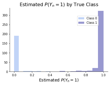
Finally, the graph below shows a distribution of the estimated \(P(Y_n = 1)\) based on each observation’s true class. This demonstrates that our model is quite confident of its predictions.
fig, ax = plt.subplots()
sns.distplot(binary_model.p[binary_model.yhat == 0], kde = False, bins = 8, label = 'Class 0', color = 'cornflowerblue')
sns.distplot(binary_model.p[binary_model.yhat == 1], kde = False, bins = 8, label = 'Class 1', color = 'darkblue')
ax.legend(loc = 9, bbox_to_anchor = (0,0,1.59,.9))
ax.set_xlabel(r'Estimated $P(Y_n = 1)$', size = 14)
ax.set_title(r'Estimated $P(Y_n = 1)$ by True Class', size = 16)
sns.despine()
Multiclass Logistic Regression
# import data
wine = datasets.load_wine()
X = wine['data']
y = wine['target']
Before fitting our multiclass logistic regression model, let’s again define some helper functions. The first (which we don’t actually use) shows a simple implementation of the softmax function. The second applies the softmax function to each row of a matrix. An example of this is shown for the matrix
The third function returns the \(I\) matrix discussed in the concept section, whose \((n, k)^\text{th}\) element is a 1 if the \(n^\text{th}\) observation belongs to the \(k^\text{th}\) class and a 0 otherwise. An example is shown for
def softmax(z):
    return np.exp(z)/(np.exp(z).sum())

def softmax_byrow(Z):
    return (np.exp(Z)/(np.exp(Z).sum(1)[:,None]))

def make_I_matrix(y):
    I = np.zeros(shape = (len(y), len(np.unique(y))), dtype = int)
    for j, target in enumerate(np.unique(y)):
        I[:,j] = (y == target)
    return I


Z_test = np.array([[1, 1],
              [0,1]])
print('Softmax for Z:\n', softmax_byrow(Z_test).round(2))

y_test = np.array([0,0,1,1,2])
print('I matrix of [0,0,1,1,2]:\n', make_I_matrix(y_test), end = '\n\n')
Softmax for Z:
 [[0.5  0.5 ]
 [0.27 0.73]]
I matrix of [0,0,1,1,2]:
 [[1 0 0]
 [1 0 0]
 [0 1 0]
 [0 1 0]
 [0 0 1]]
The multiclass logistic regression model is constructed below. After standardizing and adding an intercept, we estimate \(\hat{\mathbf{B}}\) through gradient descent. Again, we use the gradient discussed in the concept section,
class MulticlassLogisticRegression:

    def fit(self, X, y, n_iter, lr, standardize = True, has_intercept = False):

        ### Record Info ###
        if standardize:
            X = standard_scaler(X)
        if not has_intercept:
            ones = np.ones(X.shape[0]).reshape(-1, 1)
            X = np.concatenate((ones, X), axis = 1)
        self.X = X
        self.N, self.D = X.shape
        self.y = y
        self.K = len(np.unique(y))
        self.n_iter = n_iter
        self.lr = lr

        ### Fit B ###
        B = np.random.randn(self.D*self.K).reshape((self.D, self.K))
        self.I = make_I_matrix(self.y)
        for i in range(n_iter):
            Z = np.dot(self.X, B)
            P = softmax_byrow(Z)
            gradient = np.dot(self.X.T, self.I - P)
            B += lr*gradient

        ### Return Values ###
        self.B = B
        self.Z = np.dot(self.X, B)
        self.P = softmax_byrow(self.Z)
        self.yhat = self.P.argmax(1)
The multiclass model is instantiated and fit below. The yhat value returns the class with the greatest estimated probability. We are again able to classify all observations correctly.
multiclass_model = MulticlassLogisticRegression()
multiclass_model.fit(X, y, 10**4, 0.0001)
print('In-sample accuracy: '  + str(np.mean(multiclass_model.yhat == y)))
In-sample accuracy: 1.0
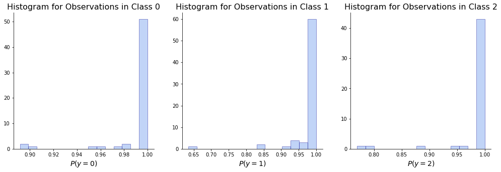
The plots show the distribution of our estimates of the probability that each observation belongs to the class it actually belongs to. E.g. for observations of class 1, we plot \(P(y_n = 1)\). The fact that most counts are close to 1 shows that again our model is confident in its predictions.
fig, ax = plt.subplots(1, 3, figsize = (17, 5))
for i, y in enumerate(np.unique(y)):
    sns.distplot(multiclass_model.P[multiclass_model.y == y, i],
                 hist_kws=dict(edgecolor="darkblue"),
                 color = 'cornflowerblue',
                 bins = 15,
                 kde = False,
                 ax = ax[i]);
    ax[i].set_xlabel(xlabel = fr'$P(y = {y})$', size = 14)
    ax[i].set_title('Histogram for Observations in Class '+ str(y), size = 16)
sns.despine()