Regression Trees
Decision trees are deeply rooted in tree-based terminology. Before discussing decision trees in depth, let’s go over some of this vocabulary.
Node: A node is comprised of a sample of data and a decision rule.
Parent, Child: A parent is a node in a tree associated with exactly two child nodes. Observations directed to a parent node are next directed to one of that parent’s two children nodes.
Rule: Each parent node has a rule that determines toward which of the child nodes an observation will be directed. The rule is based on the value of one (and only one) of an observation’s predictors.
Buds: Buds are nodes that have not yet been split. In other words, they are children that are eligible to become parents. Nodes are only considered buds during the training process. Nodes that are never split are considered leaves.
Leaf: Leaves, also known as terminal nodes, are nodes that are never split. Observations move through a decision tree until reaching a leaf. The fitted value of a test observation is determined by the training observations that land in the same leaf.
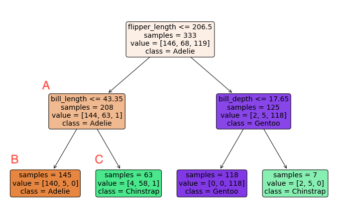
Let’s return to the tree introduced in the previous page to see these vocabulary terms in action. Each square in this tree is a node. The sample of data for node \(A\) is the collection of penguins with flipper lengths under 206.5mm and the decision rule for node \(A\) is whether the bill length is less than or equal to 43.35mm. Node \(A\) is an example of a parent node, and nodes \(B\) and \(C\) are examples of child nodes. Before node \(A\) was split into child nodes \(B\) and \(C\), it was an example of a bud. Since \(B\) and \(C\) are never split, they are examples of leaves.
The rest of this section describes how to fit a decision tree. Our tree starts with an initial node containing all the training data. We then assign this node a rule, which leads to the creation of two child nodes. Training observations are assigned to one of these two child nodes based on their response to the rule. How these rules are made is discussed in the first sub-section below.
Next, these child nodes are considered buds and are ready to become parent nodes. Each bud is assigned a rule and split into two child nodes. We then have four buds and each is once again split. We continue this process until some stopping rule is reached (discussed later). Finally, we run test observations through the tree and assign them fitted values according to the leaf they fall in.
In this section we’ll discuss how to build a tree as well as how to choose the tree’s optimal hyperparameters.
Building a Tree
Building a tree consists of iteratively creating rules to split nodes. We’ll first discuss rules in greater depth, then introduce a tree’s objective function, then cover the splitting process, and finally go over making predictions with a built tree. Suppose we have predictors \(\bx_n \in \R^D\) and a quantitative target variable \(y_n\) for \(n = 1, \dots, N\).
Defining Rules
Let’s first clarify what a rule actually is. Rules in a decision tree determine how observations from a parent node are divided between two child nodes. Each rule is based on only one predictor from the parent node’s training sample. Let \(x_{nd}\) be the \(d^\text{th}\) predictor in \(\bx_n\). If \(x_{nd}\) is quantitative, a rule is of the form
for some threshold value \(t\). If \(x_{nd}\) is categorical, a rule is of the form
where \(\mathcal{S}\) is a set of possible values of the \(d^\text{th}\) predictor.
Let’s introduce a little notation to clear things up. Let \(\mathcal{N}_m\) represent the tree’s \(m^\text{th}\) node and \(\mathcal{R}_m\) be the rule for \(\mathcal{N}_m\). Then let \(\mathcal{C}^L_m\) and \(\mathcal{C}_m^R\) be the child nodes of \(\mathcal{N}_m\). As a convention, suppose observations are directed to \(\mathcal{C}_m^L\) if they satisfy the rule and \(\mathcal{C}_m^R\) otherwise. For instance, let
Then observation \(n\) that passes through \(\mathcal{N}_m\) will go to \(\mathcal{C}_m^L\) if \(x_{n2} \leq 4\) and \(\mathcal{C}_m^R\) otherwise. On a diagram like the one above, the child node for observations satisfying the rule is often to the left while the node for those not satisfying the rule is to the right, hence the superscripts \(L\) and \(R\)
The Objective
Consider first a single node \(\mathcal{N}_m\). Let \(n \in \mathcal{N}_m\) be the collection of training observations that pass through the node and \(\bar{y}_m\) be the sample mean of these observations. The residual sum of squares (\(RSS\)) for \(\mathcal{N}_m\) is defined as
The loss function for the entire tree is the \(RSS\) across buds (if still being fit) or across leaves (if finished fitting). Letting \(I_m\) be an indicator that node \(m\) is a leaf or bud (i.e. not a parent), the total loss for the tree is written as
In choosing splits, we hope to reduce \(RSS_T\) as much as possible. We can write the reduction in \(RSS_T\) from splitting bud \(\mathcal{N}_m\) into children \(\mathcal{C}_m^L\) and \(\mathcal{C}_m^R\) as the \(RSS\) of the bud minus the sum of the \(RSS\) of its children, or
where \(\bar{y}_m^L\) and \(\bar{y}_m^R\) are the sample mean of the child nodes.
Making Splits
Finding the optimal sequence of splits to minimize \(RSS_T\) becomes a combinatorially infeasible task as we add predictors and observations. Instead, we take a greedy approach known as recursive binary splitting. When splitting each bud, we consider all possible predictors and all possible ways to split that predictor. If the predictor is quantitative, this means considering all possible thresholds for splitting. If the predictor is categorical, this means considering all ways to split the categories into two groups. After considering all possible splits, we choose the one with the greatest reduction in the bud’s \(RSS\). This process is detailed below.
Note that once a node is split, what happens to one of its children is independent of what happens to the other. We can therefore build the tree in layers—first splitting the initial node, then splitting each of the initial node’s children, then splitting all four of those children’s children, etc.
For each layer (starting with only the initial node), we split with the following process.
For each bud \(m\) on that layer,
For each predictor \(d\),
If the predictor is quantitative:
For each value of that predictor among the observations in the bud 1,
Let this value be the threshold value \(t\) and consider the reduction in \(RSS_m\) from splitting at this threshold. I.e. consider the reduction in \(RSS_m\) from the rule
\[ \mathcal{R} = x_{nd} \leq t. \]
If the predictor is categorical:
Rank the categories according to the average value of the target variable for observations in each category. If there are \(V\) distinct values, index these categories \(c_1, \dots, c_V\) in ascending order.
For \(v = 1, \dots, V-1\) 1,
Consider the set \(\mathcal{S} = \{ c_1, \dots, c_v\}\) and consider the reduction in \(RSS_m\) from the rule
\[ \mathcal{R} = x_{nd} \in \mathcal{S}. \]
In words, we consider the set of categories corresponding to the lowest average target variable and split if the observation’s \(d^\text{th}\) predictor falls in this set. We then add one more category to this set and repeat.
Choose the predictor, and value (if quantitative) or set (if categorical) with the greatest reduction in \(RSS_m\) and split accordingly.
We repeat this process until some stopping rule is reached.
Making Predictions
Making predictions with a built decision tree is very straightforward. For each test observation, we simply run the observation through the built tree. Once it reaches a leaf (a terminal node), we predict its target variable to be the sample mean of the training observations in that leaf.
Choosing Hyperparameters
As with any bias-variance tradeoff issue, we want our tree to learn valuable patterns from the data without reading into the idiosyncrasies of our particular training set. Without any sort of regulation, a tree will minimize this total \(RSS\) by moving each training observation into its own leaf, causing obvious overfitting. Below are three common methods for limiting the depth of a tree.
Size Regulation
A simple way to limit a tree’s size is to directly regulate its depth, the size of its terminal nodes, or both.
We can define the depth of a node as the number of parent nodes that have come before it. For instance, the initial node has depth 0, the children of the first split have depth 1, and the children of the second split have depth 2. We can prevent a tree from overfitting by setting a maximum depth. To do this, we simply restrict nodes of this depth from being split.
The size of a node is defined as the number of training observations in that node. We can also prevent a tree from overfitting by setting a minimum size for parent nodes or child nodes. When setting a minimum size for parent nodes, we restrict nodes from splitting if they are below a certain size. When setting a minimum size for child nodes, we ban any splits that would create child nodes smaller than a certain size.
These parameters are typically chosen with cross validation.
Minimum Reduction in RSS
Another simple method for avoiding overfitting is to require that any split decrease the residual sum of squares, \(RSS_T\), by a certain amount. Ideally, this allows the tree to separate groups that are sufficiently dissimilar while preventing it from making needless splits. Again, the exact required reduction in \(RSS_T\) should be chosen through cross validation.
One potential pitfall of this method is that early splits might elicit small decreases in \(RSS_T\) while later splits will elicit much larger ones. By requiring a minimum reduction in \(RSS_T\), however, we might not reach these later splits. For instance, consider the dataset below with input variables \(a\) and \(b\) and target variable \(y\). The first split, whether by \(a\) or \(b\), will not reduce \(RSS_T\) at all while the second split would reduce it to 0.
a |
b |
y |
|---|---|---|
0 |
0 |
0 |
0 |
1 |
10 |
1 |
0 |
10 |
1 |
1 |
0 |
Pruning
A third strategy to manage a decision tree’s size is through pruning. To prune a tree, first intentionally overfit it by, for instance, setting a low minimum node size or a high maximum depth. Then, just like pruning a literal tree, we cut back the unnecessary branches. Specifically, one by one we undue the least helpful split by re-joining terminal leaves. At any given step, we undue the split that causes the least increase in \(RSS_T\).
When pruning a tree, we want to balance tree size with residual error. Define the size of a tree (not to be confused with the size of a node) to equal its number of terminal leaves, denoted \(|T|\) for tree \(T\). The residual error for tree \(T\) is defined by \(RSS_T\). To compare possible trees when pruning, we use the following loss function
where \(\lambda\) is a regularization parameter. We choose the tree \(T\) that minimizes \(\mathcal{L}(T)\).
Increasing \(\lambda\) increases the amount of regularization and limits overfitting by penalizing larger trees. Increasing \(\lambda\) too much, however, can cause undercutting by preventing the tree from making needed splits. How then do we choose \(\lambda\)? With cross validation! Specifically, for each validation fold, we overfit the tree and prune it back using a range of \(\lambda\) values. Note that \(\lambda\) does not affect how we prune the tree, only which pruned tree we prefer. For each value of \(\lambda\), we calculate the average validation accuracy (likely using \(RSS_T\) calculated on the validation set) across folds. We choose the value of \(\lambda\) that maximizes this accuracy and the tree which is preferred by that value of \(\lambda\).
- 1(1,2)
For a quantitative predictor, we actually consider all but the largest. If we chose the rule \(R = x_{nd} \leq t\) and \(t\) was the largest value, this would not leave any observations in the second child. Similarly, for a categorical predictor, we do not consider the \(V^\text{th}\) category since this would not leave any observations for the second child.